How to Analyze and Forecast Time Series Data

With this tutorial, you will learn how to analyze and forecast time series data using various statistical and machine learning models.

What is a Time Series?

A time series is a sequence of data observed over time. For example, at specific points in time, we can observe features such as the unemployment rate of a country, sales success of a product, or demand of a certain quantity. The key is that each of these variables varies with respect to time.

Analysis of temporal data allows us to obtain useful insights on how a variable changes over time (as in a univariate time series) or how it depends on the change in the values of other variables (as in a multivariate time series). This relationship can then be further analyzed for time series forecasting (extrapolation into the future), which has numerous applications for artificial intelligence and machine learning.

Python Libraries Used for Time Series Analysis

There are several open-source Python libraries we will use for time series analysis, some of which you may have seen before. These include:

• numpy: provides fast and basic mathematical functionality on array objects
• pandas: provides highly efficient data structures such as Series and DataFrame objects
• scipy: provides functionalities for optimization, signal and image processing, integration, interpolation and linear algebra
• scikit-learn: a scipy toolkit widely used for statistical modeling, machine learning, and deep learning
• statsmodels: provides tools for statistical data exploration and modeling
• matplotlib: provides tools for data visualization in various formats (scatterplots, histograms, etc.)
• datetime: provides all the necessary functionality for reading, formatting, and manipulating time

Here’s a flowchart of some of these packages for reference: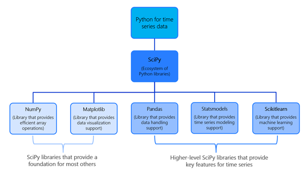

Basic Components of a Time Series

A time series is comprised of four basic components:

• Level: the mean value around which the time series varies
• Trend: the increasing or decreasing behavior of a variable over time
• Seasonality: any cyclic behavior of a variable over time
• Noise/Residual: the remaining error in the observations (due to environmental factors)

It is helpful to think of these four components as combining either additively or multiplicatively. An additive model suggests that these components are added together

[y(t) = Level + Trend + Seasonality + Noise]

while a multiplicative model suggests that the components are multiplied together.

[y(t) = Level * Trend * Seasonality * Noise]. 

This decompositional approach to time series provides a structured way to think about forecasting problems, both generally in terms of modeling complexity and specifically in terms of how best to represent each of these components within a given model.

However, you may not always be able to perfectly break down your time series into an additive or multiplicative model. Unfortunately, real-world problems are messy and noisy. A time series could consist of both additive and multiplicative components. There could be an increasing trend, followed by a decreasing trend. In spite of this, abstract models provide a simple framework by which you can analyze your data and explore ways to look at and forecast your problem.

Time Series Decomposition Using Statsmodels

import pandas as pd
import matplotlib.pyplot as plt
from statsmodels.tsa.seasonal import seasonal_decompose
series = pd.read_csv('FILENAME')
result = seasonal_decompose(series, model='multiplicative') # can use additive as well
result.plot()
plt.show()

Terms Used in Forecasting

Here are several universal terms we will use when discussing forecasting:

• forecast: Forecasting involves predicting values in the future, where “future” is defined as observations that occur after the data used to train the model
• fitted values: These are predictions made by the time series model on the training data
• train/test split: This involves splitting the data into training data (used to develop the model) and testing data (used to evaluate model performance). Unlike many other machine learning models, this process is not random. Instead, we set a cutoff point and let observations that occur before this cutoff constitute the training data, and those after the cutoff the testing data.

Common Models Used for Time Series Forecasting

We have a few naive heuristics for simple forecasting:

• “Most Recent”/Naive Method: For these methods, we simply set all forecasts to be the value of the last observation.
• “Average”/Mean Method: Here, the forecasts of all future values are simply equal to the average of the historical training data.
• Seasonal Naive Method: This naive method is particularly useful for seasonal data. We set each forecast to be the last observed value from the same season.

Exponential Smoothing

Exponential smoothing has motivated some of the most successful forecasting models. The idea is that recent examples are weighted averages of previous observations, with the weights decaying exponentially as the observations get older. Generally, there are several different types of exponential smoothing, but we will focus on two: simple exponential smoothing (SES), and Holt-Winters.

Simple Exponential Smoothing

This method is suitable for forecasting data with no clear trend or seasonal pattern. As we saw with the “Most Recent” method and the “Average” method, forecasts were dependent on some weighted average of the observed data (in the “Most Recent” method, all of the weight is given to the last observation, while in the “Average” method, all observations have equal importance). We often want some balance between these two situations: one where we can attach larger weights to more recent observations, but still significantly consider a window of recent observations when determining forecasted values. SES is one way to accomplish this.

In SES, the forecast at time $T+1$ is equal to the weighted average between the most recent observation $y_T$ and the previous forecast $ŷ_{T-1 \vert T }$. More formally:

where $0\leq \alpha \leq 1$ is a smoothing parameter. For the fitted values (one-step forecasts of the training data), we can similarly write them as:

for $t=1, 2, … , T$. We can use this recursive definition to write an expression for the forecast at time $T + 1$ in terms of all previous observations, namely:

We can now see how the weights of observations decrease as they get older. Older observations correspond to a larger value of i, which increases the exponent of the $1-\alpha$ coefficient of the observation. And since $0\leq 1-\alpha \leq 1$, increasing the exponent of $1-\alpha$ decreases the value of $(1-\alpha)^i$.

How do we choose $\alpha$? In some cases, we can choose it in a subjective matter, specified based on previous experience. However, a more generally reliable and objective approach is to estimate it from observed data. Just like in many machine learning models, this involves minimizing a loss function applied on the training data. So we can obtain a good value of by choosing the one that minimizes some loss function (generally, the sum of the squared errors).

An unfortunate downfall of SES is the “flat-forecast” function. In other words, all forecasts take the same value, equal to the last level component, namely:

for $h=2, 3, …$ Hence, these forecasts are only suitable if the time series has no trend or seasonality, but can also be useful as a baseline.

Fortunately, Python can implement Simple Exponential Smoothing using statsmodels.

from statsmodels.tsa.api import SimpleExpSmoothing

n = len(series)
cutoff = int(0.5*n) # determines split of training and testing data
series_train = series[:cutoff]
series_test = series[cutoff:]

h = len(series_test) # number of forecast predictions you want to make
fit = SimpleExpSmoothing(series_train).fit()
series_hat = fit.fitted_values
forecast = fit.forecast(h)

# Plotting
plt.scatter(range(n), series)
plt.plot(range(cutoff), series_hat)
forecast.plot()

Holt-Winters Model

Often, our time series data has inherent trend and seasonality, and SES tends to perform poorly on such models. At a high-level, Holt-Winters applies seasonality three times:

• Level smoothing (with parameter $\alpha$)
• Trend smoothing (with parameter $\beta$)
• Seasonal smoothing (with parameter $\gamma$)

We also specify the length of a seasonal period ($s$). Additionally, we can specify whether or not to explore seasonality as additive or multiplicative in nature.

Holt-Winters Additive Holt-Winters Multiplicative Model: Model: Updating: Updating: When to use: When to use:

Autoregressive Models

For stationary time series (i.e., no trend and seasonality), an autoregression sees the value of a variable at time $t$ as a linear function of the values preceding it. Mathematically, this can be expressed as:

In the above expression, $p$ is the autoregressive parameter which indicates how many time steps to look at previously. $\epsilon_t$ is white noise, meaning that errors are independent and identically distributed (i.i.d) with a normal distribution that has mean 0 and constant variance.

The value of $p$ can be set using various approaches, but one common method is to look at the auto-correlation function (ACF) plot or correlogram. This graph is a visual way to show serial correlation in data at various lags. The statsmodels library allows us to visualize the autocorrelation plot:

from statsmodels.graphics.tsaplots import plot_acf

cutoff = int(0.5*n) # determines split of training and testing data
series_train = series[:cutoff] # divides time series into training and testing
series_test = series[cutoff:]
plot_acf(series_train, lags = 100)
plt.show()

Moving Average Models

For stationary time series, a moving average model will, similar to an autoregressive model, model the value of a variable as a linear combination of previous information. However, rather than using the values of the observations, a moving average will use the residual errors. Specifically:

where $q$ is the moving average parameter, $\epsilon_t$ is white noise, and $\epsilon_{t-1} … \epsilon_{t-q}$ are the error terms at previous time periods.

The value of $q$ can be set using various approaches, but one common method is to look at the partial auto-correlation function (PACF) plot. A PACF plot is similar to an ACF plot in that we look at correlation values across different lags, except that in a PACF, each partial correlation controls for any correlation between observations of a shorter lag length. Here is how we can plot a PACF using statsmodels (note the code is very similar!):

from statsmodels.graphics.tsaplots import plot_pacf

cutoff = int(0.5*n) # determines split of training and testing data
series_train = series[:cutoff] # divides time series into training and testing
series_test = series[cutoff:]
plot_pacf(series_train, lags = 100)
plt.show()