Networks Analysis

A Beginner’s Guide To What It Is, How To Implement It, and Why It Matters.

Things to Know Before Reading

Just to be transparent with what this tutorial aims to accomplish, this is by no means a comprehensive tutorial over networks. This tutorial aims to introduce to beginners the concept of networks, some important and common terminology, as well as some code to get you started with the proper directions to explore the vast world of networks on your own. Each of the sections below have a text and code toggle for you to examine the code used to make these simple network graphs. The Python library used here is networkx (documentation can be found here). D3.js is also a popular language for making beautiful and dynamic network graphs (and visualizations in general) but can be slightly trickier to learn. Enjoy the tutorial and stick around at the end for further recommended resources!

Nodes

Technical Description

A node (or vertex) is the most fundamental unit on which graphs are based. In graph theory, they may also be referred to as “point”, “junction”, or “0 - simplex”.

Real-World Relevance

This single datapoint could be interpreted in different ways depending on the context. If you were to consider a network of the human race, each node would be a person. For the network of webpages on the world wide web, each node would be a webpage. A node could also represent a single train station in a somewhat complex railway network. It is important to note that while we typically consider a node to be the fundamental unit of graphs, each node itself could contain a lot of information. In a social network, where each node represents a person, each node is a user profile comprised of data about the user’s gender, age, contact information, their preferences, and other information they have made public.

Edges

Technical Description

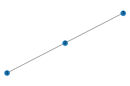
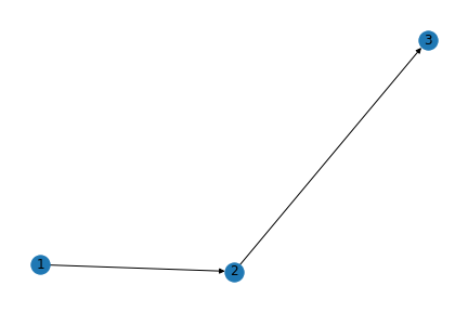
The links with which two nodes are connected to each other are called edges. In this case, for example, there are 3 nodes and 2 edges (one connects Node 1 and Node 2, and the other connects Node 2 and Node 3). The nodes that an edge connects are called neighbors. Note that Node 1 and Node 3 aren’t neighbors with each other here. Broadly, we can have either undirected or directed graphs based on the context. In directed graphs (to the right), a node connects to another with a directed edge, indicating an asymmetric relationship.

In the case of undirected graphs (to the right), an undirected edge implies a symmetric relationship between the two nodes it connects.

Real-World Relevance

An edge implies a relationship between the two entities, which are repsented by nodes. In a social network, for example, an edge could imply a connection between two people. The nuance of directed and undirected graphs gives us a convenient way to represent more complex information. For example, a directed graph would be more fitting if we were to represent a genealogy network - we can then direct edges from ancestors to their successors (since it is somewhat an asymmetric relationship). Even a social network, which you would typically represent as an undirected graph, could be represented as a directed graph if you were to consider who sent whom the friend/follow request first - this would add another interesting dimension to the problem.

Paths, Cycles, Connectivity

Technical Description

Path: A path is a sequence of nodes where “each consecutive pair in the sequence is connected with an edge” (Easley and Kleinberg, 2010). Broadly, if a path does not repeat any nodes, it is called a simple path. If it doesn’t repeat any nodes, it is a non-simple path. In graph theory, a path is a trail in which all vertices (and edges) are distinct. In our example, there is a clear path from 1 to 3, and from 3 to 1 (via 2).

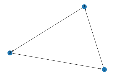
Cycle: A cycle is a non-simple path with “at-least three edges, in which the first and last nodes are the same, but otherwise all nodes are distinct” (Easley and Kleinberg, 2010). A cycle graph is a graph of a cycle which has no repeated vertices and edges (a simple cycle). The given visualization is an example of a cycle graph.

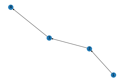
A commonly-used concept is that of a Directed Acyclical Graph (DAG), which is what the name implies - a graph that is acyclical in nature (does not have the same first and last nodes) and has directed edges. The given visualization represents a simple DAG with four nodes (1, 2, 3, 4).

Connectivity: A graph is said to be connected “if for every pair of nodes, there is a path between them” (Easley and Kleinberg, 2010). In other words, there is a way to get from each node to each other node (regardless of how simple or complex that route may be).

Real-World Relevance

Paths and connectivity could be understood together. If we wanted to see if two nodes are connected, we could check if there exists a path between them. Consider the case of a police chasing a criminal on the run - traditionally, they would not be connected with the criminal and their job is to find a path (the shortest, most efficient one) to the criminal. They would conduct an investigation, find who are closest to the criminal (the end node), and trace back connections to one they could directly inquire. As soon as they find a link with the criminal, they are then connected to the criminal in the sense of a network, and can pursue the path. In short, unless they are connected to the end node, they do not have a viable path to pursue. Directed acylical graphs are also easy to understand in context of your daily lives. For example, consider what you have done today - likely, you brushed your teeth after you woke up, after which you probably (hopefully) had breakfast. This can be represented as a DAG, since each subsequent event (or node) has a dependency on the previous one. You can only brush your teeth after you woke up, and so you would draw a directed edge from “waking up” to “brushing teeth”.

Distance of Six Degrees of Separation

Technical Description

Distance: The distance between any two nodes in a graph is the “length of the shortest path between them” (Easley and Kleinberg, 2010). In our example, there the distance from node 1 to node 3 is 2. Sometimes, however, graphs are more complex and it is harder to compute the distance - this is where Breadth First Search and Depth First Search are useful.

Real-World Relevance

As the access to internet improves worldwide, the world is more connected than ever. Therefore, the idea of “six degrees of separation” is more relevant than ever. This idea states that all people are at-most six social connections away from each other. While the notion grew out of Stanley Milgram’s work in the 1960s, (a lot of work) has been done on the subject since.

Triadic Closure

Technical Description

Triadic Closure: The Triadic Closure principle underlines the evolving nature of networks, and states the following: “If two people in a social network have a friend in common, then there is an increased likelihood that they will become friends themselves at some point in the future” (Easley and Kleinberg, 2010). In our example, the Triadic Closure Principle hypothesizes that if 2 is friends with both 1 and 3, there is an increased likelihood that 1 and 3 would also be friends. This is displayed in the second iteration (triangular-looking closed graph - hence the name “triadic closure”) of the same group of nodes. “Triadic closure is intuitively very natural, and essentially everyone can find examples from their own experience. Moreover, experience suggests some of the basic reasons why it operates. One reason why B and C are more likely to become friends, when they have a common friend A, is simply based on the opportunity for B and C to meet: if A spends time with both B and C, then there is an increased chance that they will end up knowing each other and potentially becoming friends. A second, related reason is that in the process of forming a friendship, the fact that each of B and C is friends with A (provided they are mutually aware of this) gives them a basis for trusting each other that an arbitrary pair of unconnected people might lack.” (Easley and Kleinberg, 2010).

Real-World Relevance

“Triadic closure is intuitively very natural, and essentially everyone can find examples from their own experience. Moreover, experience suggests some of the basic reasons why it operates. One reason why B and C are more likely to become friends, when they have a common friend A, is simply based on the opportunity for B and C to meet: if A spends time with both B and C, then there is an increased chance that they will end up knowing each other and potentially becoming friends. A second, related reason is that in the process of forming a friendship, the fact that each of B and C is friends with A (provided they are mutually aware of this) gives them a basis for trusting each other that an arbitrary pair of unconnected people might lack.” (Easley and Kleinberg, 2010).

Measures of Centrality

Technical Description

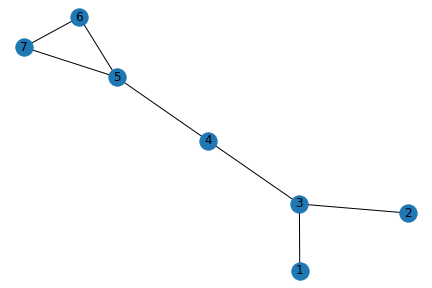
Degree Centrality: The degree centrality of a node refers to the number of edges that are attached to that node. This score can be standardized by dividing the score for each node by n - 1, where n is the total number of nodes in the network. Let’s consider node 5 in the graph below. There are 3 edges connected to the node, and 7 nodes in the graph in total. Therefore, the standardized degree centrality for node 5 is 3/(7-1) = 0.5.

Betweenness Centrality: The betweenness centrality of a node refers to the number of times that node lies on the shortest path between other nodes. This score can be standardized by dividing these scores by (n-1)(n-2)/2 (for undirected graphs) for each node, where n is the total number of nodes in the network.

Closeness Centrality: The closeness centrality of a node depends on the sum of its shortest paths to all other nodes. In mathematical terms, it is the inverse of the sum of shortest paths of a node to all other nodes). It can be standardized by multiplying the result by n - 1, where n is the total number of nodes in the network. In our graph above, the standardized score for the closeness centrality of node 5 is 1/11 * (7 - 1) = 6/11.

Embeddedness

Technical Description

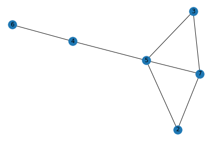
Embeddedness: The embeddedness of an edge refers to the number of common neighbors that the two nodes at the end of the edge have. (Easley and Kleinberg, 2010). In our example, nodes 5 and 7 have both node 3 and node 2 in common. Therefore, the embeddedness of the A-B edge is 2.

Real-World Relevance

“A long line of research in sociology has argued that if two individuals are connected by an embedded edge, then this makes it easier for them to trust one another, and to have confidence in the integrity of the transactions (social, economic, or otherwise) that take place between them. Indeed, the presence of mutual friends puts the interactions between two people “on display” in a social sense, even when they are carried out in private; in the event of misbehavior by one of the two parties to the interaction, there is the potential for social sanctions and reputational consequences from their mutual friends…No similar kind of deterring threat exists for edges with zero embeddedness, since there is no one who knows both people involved in the interaction. “ (Easley and Kleinberg, 2010).

Homophily

Technical Description

Homophily in the context of social networks refers to the idea that we tend to be similar to our friends in all manners of characteristics, ranging from age, race, affluence, etc (Easely and Kleinberg 2010).

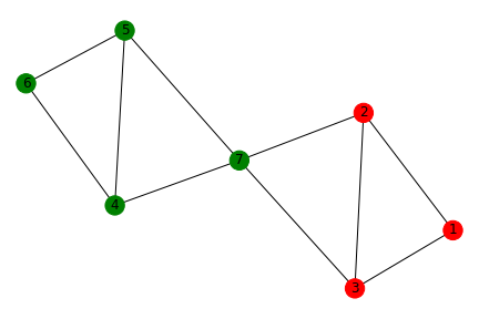
In this example, we see that this is an easily identifiable case of homophily with the only connection between the two groups of nodes being node 7 (which connects to nodes 2 and 3). We can determine this more precisely if the fraction of heterogeneous edges is significantly less than the likelihood of a heterogeneous edge forming, then it’s a case of homophily. Here, we have 2 groups (denoted as red and green) with their likelihood of appearing being 3/7 and 4/7 respectively, making the likelihood of a heterogeneous edge 2(3/7)(4/7) = 24/49. However, the fraction of heterogeneous edges is actually 2/10, far less than 24/49. Conversely, when the fraction of heterogeneous edges is significantly larger than the likelihood of heterogeneous edges forming, it would be inverse homophily.

Revisiting Triadic Closure, we can likely say that node 6 has similar characteristics as nodes 4 and 5 due to homophily, and even though nodes 4 and 5 are not connected and hypothetically don’t know that they are both mutually connected with node 6, they are still very likely to be similar and even form a connection.

Real-World Relevance

You can find these relations everywhere in life, from social and political echo chambers, friend circles, parties, coworkers. Many of your friends or coworkers will probably share similar socio-political values as you or share the same income bracket or same age etc. This is by no means a hard rule but simply highlights the fact that the chance of people forming connections is most likely explained by the fact that they shared something in common to begin with. This is also a manifestation of the phrase: “Birds of a feather, flock together”. A very interesting outcome of Homophily is with segregation. An American economist Thomas Schelling made some interesting revelations regarding this (which can be found here.)

Propinquity

Technical Description

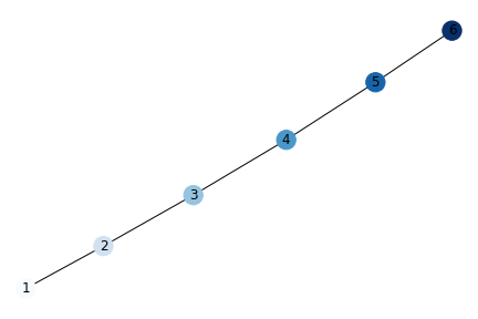
In a similar vein as Homophily, Propinquity is the idea that we tend to have shared characteristics or connections with those we are in geographical proximity with. The same principles discussed in Homophily can also apply to Propinquity. As you can see from the example, the edges represent physical location and nodes closer to each other share a more similar shade of blue than those farther away, illustrating the strength of connections due to geographic location.

Real-World Relevance

Think of the friends you first made in college, most likely people who shared the same dorm right? Or even closer, the same hallway? The friends you made in your childhood/teenage years all probably lived near you as you all went to the same school/church/activities. There have also been studies that show professors collaborating more with those who share the same space/building. These ideas are just a formation of common observations we see about our circles and networks in every day life.

Affiliation

Technical Description

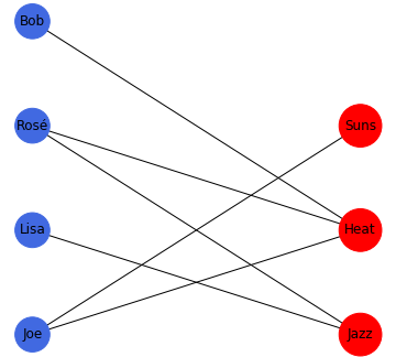
So far, we have been describing the characteristics of nodes as some external factor either not shown in graphs or represented as different colors in the last few examples. In affiliation networks, these characteristics, also known as foci, are nodes themselves in addition to the standard nodes. These network graphs can take several forms. Bipartite graphs separate the foci from the actors/people. In this example you can see which Basketball teams in the NBA that Lisa, Rosé, Joe, and Bob are a fan of respectively.

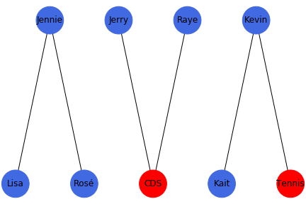
Social-Affiliation Networks combine these foci and nodes into a standard network graph, displaying both relations from actors to other actors as well as actors to foci. Revisiting Triadic Closure once more, we can apply the concept onto social-affiliation networks as well. For example, traditional Triadic Closure expects that given a pair of friendships: Jen & Lisa, Jen & Rosé, we can expect that Lisa & Rosé will become friends. When the shared connection is a foci, it is called a Focal Closure. Such is the case where Jerry and Raye are both part of Cornell Data Science and thus are likely to form a connection at some point. When the shared connection between an actor/person and a foci is an actor/person, it’s called a Membership Closure. If Kevin plays tennis and is friends with Kait, there is a reasonable chance that Kevin introduces Kait to playing Tennis.

Balance

Technical Description

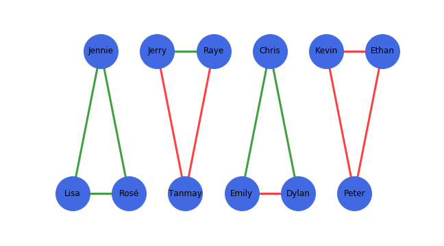
In the context of social networks, we can add further detail to edges i.e. positive (+) and negative (-) (denoted as green and red edges in our examples) relations between nodes, and due to pyschology and social dynamics, certain orientations of these relations are more plausible than others (stable/balanced relationships). In life, if an unstable/unbalanced relationship exists, social forces due to stress or psychological dissonance will try to correct this. We can see in these examples that the only balanced relationships occur when all 3 people are friends or 2 people are friends and mutual enemies of a third. In the event that a person is mutual friends with two enemies then they will try and reconcile this relationship as it incurs stress upon that person (unstable). Similarly, if all 3 people are enemies then the saying “the enemy of my enemy is my friend” may occur and two individuals will become friends to avoid the “Mexican Standoff” scenario (again unstable).

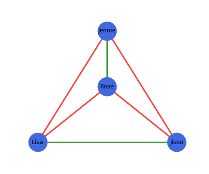
From these examples we can define a formal property of a structurally balanced graph: “For every set of three nodes, if we consider the three edges connecting them, either all three of these edges are labeled +, or else exactly one of them is labeled +” (Easely and Kleinberg 2010). Using this, we can properly identify the example to the right as balanced.

Real-World Relevance

The implications of balancing social networks is something we deal with on a daily basis, since as social creatures, we try to maintain balance as much as possible and minimize any sources of instability within our friendships. This can also be applied to relations amongst public (and potentially political) figures and foreign relations between countries.

Resources and Final Words

Here are some useful resources to continue learning about network analysis:

• (A more comprehensive overview of the basics with a wider array of examples of code)
• (A neat side project for visualizing a network graph of your Facebook friends)
• (Learn how to make network graphs in R)
• (Learn how to make network graphs in D3)

References Used in This Tutorial:

• Easley, David, and Jon Kleinberg. (Networks, crowds, and markets. Vol. 8). Cambridge: Cambridge university press, 2010.
• Weisstein, Eric W. “Graph Vertex.” From MathWorld–A Wolfram Web Resource. [(https://mathworld.wolfram.com/GraphVertex.html)]
• Bender, Edward A., and S. Gill Williamson. (Lists, Decisions and Graphs). S. Gill Williamson, 2010.
• Morse, Gardiner. (The Science Behind Six Degrees). Harvard Business Review, 2003.
• Watabe, Motoki. [(https://www.sscnet.ucla.edu/soc/faculty/mcfarland/soc112/cent-ans.htm)]. 1998.